Tutorial - What is a variational autoencoder?
Understanding Variational Autoencoders (VAEs) from two perspectives: deep learning and graphical models.
Why do deep learning researchers and probabilistic machine learning folks get confused when discussing variational autoencoders? What is a variational autoencoder? Why is there unreasonable confusion surrounding this term?
There is a conceptual and language gap. The sciences of neural networks and probability models do not have a shared language. My goal is to bridge this idea gap and allow for more collaboration and discussion between these fields, and provide a consistent implementation (Github link). If many words here are new to you, jump to the glossary.
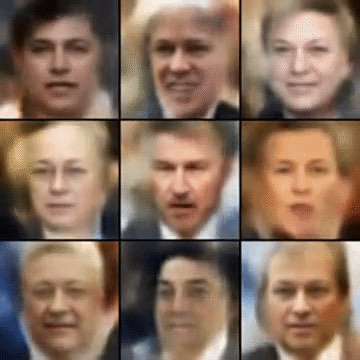
Variational autoencoders are cool. They let us design complex generative models of data, and fit them to large datasets. They can generate images of fictional celebrity faces and high-resolution digital artwork.
These models also yield state-of-the-art machine learning results in image generation and reinforcement learning. Variational autoencoders (VAEs) were defined in 2013 by Kingma et al. and Rezende et al..
How can we create a language for discussing variational autoencoders? Let’s think about them first using neural networks, then using variational inference in probability models.
The neural net perspective
In neural net language, a variational autoencoder consists of an encoder, a decoder, and a loss function.

The encoder is a neural network. Its input is a datapoint \(x\), its output is a hidden representation \(z\), and it has weights and biases \(\theta\). To be concrete, let’s say \(x\) is a 28 by 28-pixel photo of a handwritten number. The encoder ‘encodes’ the data which is \(784\)-dimensional into a latent (hidden) representation space \(z\), which is much less than \(784\) dimensions. This is typically referred to as a ‘bottleneck’ because the encoder must learn an efficient compression of the data into this lower-dimensional space. Let’s denote the encoder \(q_\theta (z \mid x)\). We note that the lower-dimensional space is stochastic: the encoder outputs parameters to \(q_\theta (z \mid x)\), which is a Gaussian probability density. We can sample from this distribution to get noisy values of the representations \(z\).
The decoder is another neural net. Its input is the representation \(z\), it outputs the parameters to the probability distribution of the data, and has weights and biases \(\phi\). The decoder is denoted by \(p_\phi(x\mid z)\). Running with the handwritten digit example, let’s say the photos are black and white and represent each pixel as \(0\) or \(1\). The probability distribution of a single pixel can be then represented using a Bernoulli distribution. The decoder gets as input the latent representation of a digit \(z\) and outputs \(784\) Bernoulli parameters, one for each of the \(784\) pixels in the image. The decoder ‘decodes’ the real-valued numbers in \(z\) into \(784\) real-valued numbers between \(0\) and \(1\). Information from the original \(784\)-dimensional vector cannot be perfectly transmitted, because the decoder only has access to a summary of the information (in the form of a less-than-\(784\)-dimensional vector \(z\)). How much information is lost? We measure this using the reconstruction log-likelihood \(\log p_\phi (x\mid z)\) whose units are nats. This measure tells us how effectively the decoder has learned to reconstruct an input image \(x\) given its latent representation \(z\).
The loss function of the variational autoencoder is the negative log-likelihood with a regularizer. Because there are no global representations that are shared by all datapoints, we can decompose the loss function into only terms that depend on a single datapoint \(l_i\). The total loss is then \(\sum_{i=1}^N l_i\) for \(N\) total datapoints. The loss function \(l_i\) for datapoint \(x_i\) is:
\[l_i(\theta, \phi) = - \mathbb{E}_{z\sim q_\theta(z\mid x_i)}[\log p_\phi(x_i\mid z)] + \mathbb{KL}(q_\theta(z\mid x_i) \mid\mid p(z))\]The first term is the reconstruction loss, or expected negative log-likelihood of the \(i\)-th datapoint. The expectation is taken with respect to the encoder’s distribution over the representations. This term encourages the decoder to learn to reconstruct the data. If the decoder’s output does not reconstruct the data well, statistically we say that the decoder parameterizes a likelihood distribution that does not place much probability mass on the true data. For example, if our goal is to model black and white images and our model places high probability on there being black spots where there are actually white spots, this will yield the worst possible reconstruction. Poor reconstruction will incur a large cost in this loss function.
The second term is a regularizer that we throw in (we’ll see how it’s derived later). This is the Kullback-Leibler divergence between the encoder’s distribution \(q_\theta(z\mid x)\) and \(p(z)\). This divergence measures how much information is lost (in units of nats) when using \(q\) to represent \(p\). It is one measure of how close \(q\) is to \(p\).
In the variational autoencoder, \(p\) is specified as a standard Normal distribution with mean zero and variance one, or \(p(z) = Normal(0,1)\). If the encoder outputs representations \(z\) that are different than those from a standard normal distribution, it will receive a penalty in the loss. This regularizer term means ‘keep the representations \(z\) of each digit sufficiently diverse’. If we didn’t include the regularizer, the encoder could learn to cheat and give each datapoint a representation in a different region of Euclidean space. This is bad, because then two images of the same number (say a 2 written by different people, \(2_{alice}\) and \(2_{bob}\)) could end up with very different representations \(z_{alice}, z_{bob}\). We want the representation space of \(z\) to be meaningful, so we penalize this behavior. This has the effect of keeping similar numbers’ representations close together (e.g. so the representations of the digit two \({z_{alice}, z_{bob}, z_{ali}}\) remain sufficiently close).
We train the variational autoencoder using gradient descent to optimize the loss with respect to the parameters of the encoder and decoder \(\theta\) and \(\phi\). For stochastic gradient descent with step size \(\rho\), the encoder parameters are updated using \(\theta \leftarrow \theta - \rho \frac{\partial l}{\partial \theta}\) and the decoder is updated similarly.
The probability model perspective
Now let’s think about variational autoencoders from a probability model perspective. Please forget everything you know about deep learning and neural networks for now. Thinking about the following concepts in isolation from neural networks will clarify things. At the very end, we’ll bring back neural nets.
In the probability model framework, a variational autoencoder contains a specific probability model of data \(x\) and latent variables \(z\). We can write the joint probability of the model as \(p(x, z) = p(x \mid z) p(z)\). The generative process can be written as follows.
For each datapoint \(i\):
- Draw latent variables \(z_i \sim p(z)\)
- Draw datapoint \(x_i \sim p(x\mid z)\)
We can represent this as a graphical model:
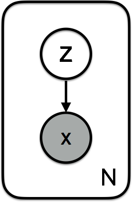
This is the central object we think about when discussing variational autoencoders from a probability model perspective. The latent variables are drawn from a prior \(p(z)\). The data \(x\) have a likelihood \(p(x \mid z)\) that is conditioned on latent variables \(z\). The model defines a joint probability distribution over data and latent variables: \(p(x, z)\). We can decompose this into the likelihood and prior: \(p(x,z) = p(x\mid z)p(z)\). For black and white digits, the likelihood is Bernoulli distributed.
Now we can think about inference in this model. The goal is to infer good values of the latent variables given observed data, or to calculate the posterior \(p(z \mid x)\). Bayes says:
\[p(z \mid x) = \frac{p(x \mid z)p(z)}{p(x)}.\]Examine the denominator \(p(x)\). This is called the evidence, and we can calculate it by marginalizing out the latent variables: \(p(x) = \int p(x \mid z) p(z) dz\). Unfortunately, this integral requires exponential time to compute as it needs to be evaluated over all configurations of latent variables. We therefore need to approximate this posterior distribution.
Variational inference approximates the posterior with a family of distributions \(q_\lambda(z \mid x)\). The variational parameter \(\lambda\) indexes the family of distributions. For example, if \(q\) were Gaussian, it would be the mean and variance of the latent variables for each datapoint \(\lambda_{x_i} = (\mu_{x_i}, \sigma^2_{x_i}))\).
How can we know how well our variational posterior \(q(z \mid x)\) approximates the true posterior \(p(z \mid x)\)? We can use the Kullback-Leibler divergence, which measures the information lost when using \(q\) to approximate \(p\) (in units of nats):
\[\mathbb{KL}(q_\lambda(z \mid x) \mid \mid p(z \mid x)) =\] \[\mathbf{E}_q[\log q_\lambda(z \mid x)]- \mathbf{E}_q[\log p(x, z)] + \log p(x)\]Our goal is to find the variational parameters \(\lambda\) that minimize this divergence. The optimal approximate posterior is thus
\[q_\lambda^* (z \mid x) = {\arg\min}_\lambda \mathbb{KL}(q_\lambda(z \mid x) \mid \mid p(z \mid x)).\]Why is this impossible to compute directly? The pesky evidence \(p(x)\) appears in the divergence. This is intractable as discussed above. We need one more ingredient for tractable variational inference. Consider the following function:
\[ELBO(\lambda) = \mathbf{E}_q[\log p(x, z)] - \mathbf{E}_q[\log q_\lambda(z \mid x)].\]Notice that we can combine this with the Kullback-Leibler divergence and rewrite the evidence as
\[\log p(x) = ELBO(\lambda) + \mathbb{KL}(q_\lambda(z \mid x) \mid \mid p(z \mid x))\]By Jensen’s inequality, the Kullback-Leibler divergence is always greater than or equal to zero. This means that minimizing the Kullback-Leibler divergence is equivalent to maximizing the ELBO. The abbreviation is revealed: the Evidence Lower BOund allows us to do approximate posterior inference. We are saved from having to compute and minimize the Kullback-Leibler divergence between the approximate and exact posteriors. Instead, we can maximize the ELBO which is equivalent (but computationally tractable).
In the variational autoencoder model, there are only local latent variables (no datapoint shares its latent \(z\) with the latent variable of another datapoint). So we can decompose the ELBO into a sum where each term depends on a single datapoint. This allows us to use stochastic gradient descent with respect to the parameters \(\lambda\) (important: the variational parameters are shared across datapoints - more on this here). The ELBO for a single datapoint in the variational autoencoder is:
\[ELBO_i(\lambda) = \mathbb{E}{q_\lambda(z\mid x_i)}[\log p(x_i\mid z)] - \mathbb{\mathbb{KL}}(q_\lambda(z\mid x_i) \mid\mid p(z)).\]To see that this is equivalent to our previous definition of the ELBO, expand the log joint into the prior and likelihood terms and use the product rule for the logarithm.
Let’s make the connection to neural net language. The final step is to parametrize the approximate posterior \(q_\theta (z \mid x, \lambda)\) with an inference network (or encoder) that takes as input data \(x\) and outputs parameters \(\lambda\). We parametrize the likelihood \(p(x \mid z)\) with a generative network (or decoder) that takes latent variables and outputs parameters to the data distribution \(p_\phi(x \mid z)\). The inference and generative networks have parameters \(\theta\) and \(\phi\) respectively. The parameters are typically the weights and biases of the neural nets. We optimize these to maximize the ELBO using stochastic gradient descent (there are no global latent variables, so it is kosher to minibatch our data). We can write the ELBO and include the inference and generative network parameters as:
\[ELBO_i(\theta, \phi) = \mathbb{E}{q_\theta(z\mid x_i)}[\log p_\phi(x_i\mid z)] - \mathbb{KL}(q_\theta(z\mid x_i) \mid\mid p(z)).\]This evidence lower bound is the negative of the loss function for variational autoencoders we discussed from the neural net perspective; \(ELBO_i(\theta, \phi) = -l_i(\theta, \phi)\). However, we arrived at it from principled reasoning about probability models and approximate posterior inference. We can still interpret the Kullback-Leibler divergence term as a regularizer, and the expected likelihood term as a reconstruction ‘loss’. But the probability model approach makes clear why these terms exist: to minimize the Kullback-Leibler divergence between the approximate posterior \(q_\lambda(z \mid x)\) and model posterior \(p(z \mid x)\).
What about the model parameters? We glossed over this, but it is an important point. The term ‘variational inference’ usually refers to maximizing the ELBO with respect to the variational parameters \(\lambda\). We can also maximize the ELBO with respect to the model parameters \(\phi\) (e.g. the weights and biases of the generative neural network parameterizing the likelihood). This technique is called variational EM (expectation maximization), because we are maximizing the expected log-likelihood of the data with respect to the model parameters.
That’s it! We have followed the recipe for variational inference. We’ve defined:
- a probability model \(p\) of latent variables and data
- a variational family \(q\) for the latent variables to approximate our posterior
Then we used the variational inference algorithm to learn the variational parameters (gradient ascent on the ELBO to learn \(\lambda\)). We used variational EM for the model parameters (gradient ascent on the ELBO to learn \(\phi\)).
Experiments
Now we are ready to look at samples from the model. We have two choices to measure progress: sampling from the prior or the posterior. To give us a better idea of how to interpret the learned latent space, we can visualize what the posterior distribution of the latent variables \(q_\lambda(z \mid x)\) looks like.
Computationally, this means feeding an input image \(x\) through the inference network to get the parameters of the Normal distribution, then taking a sample of the latent variable \(z\). We can plot this during training to see how the inference network learns to better approximate the posterior distribution, and place the latent variables for the different classes of digits in different parts of the latent space. Note that at the start of training, the distribution of latent variables is close to the prior (a round blob around \(0\)).
We can also visualize the prior predictive distribution. We fix the values of the latent variables to be equally spaced between \(-3\) and \(3\). Then we can take samples from the likelihood parametrized by the generative network. These ‘hallucinated’ images show us what the model associates with each part of the latent space.
Glossary
We need to decide on the language used for discussing variational autoencoders in a clear and concise way. Here is a glossary of terms I’ve found confusing:
- Variational Autoencoder (VAE): in neural net language, a VAE consists of an encoder, a decoder, and a loss function. In probability model terms, the variational autoencoder refers to approximate inference in a latent Gaussian model where the approximate posterior and model likelihood are parametrized by neural nets (the inference and generative networks).
- Loss function: in neural net language, we think of loss functions. Training means minimizing these loss functions. But in variational inference, we maximize the ELBO (which is not a loss function). This leads to awkwardness like calling
optimizer.minimize(-elbo)as optimizers in neural net frameworks only support minimization. - Encoder: in the neural net world, the encoder is a neural network that outputs a representation \(z\) of data \(x\). In probability model terms, the inference network parametrizes the approximate posterior of the latent variables \(z\). The inference network outputs parameters to the distribution \(q(z \mid x)\).
- Decoder: in deep learning, the decoder is a neural net that learns to reconstruct the data \(x\) given a representation \(z\). In terms of probability models, the likelihood of the data \(x\) given latent variables \(z\) is parametrized by a generative network. The generative network outputs parameters to the likelihood distribution \(p(x \mid z)\).
- Local latent variables: these are the \(z_i\) for each datapoint \(x_i\). There are no global latent variables. Because there are only local latent variables, we can easily decompose the ELBO into terms \(\mathcal{L}_i\) that depend only on a single datapoint \(x_i\). This enables stochastic gradient descent.
- Inference: in neural nets, inference usually means prediction of latent representations given new, never-before-seen datapoints. In probability models, inference refers to inferring the values of latent variables given observed data.
One jargon-laden concept deserves its own subsection:
Mean-field versus amortized inference
This issue was very confusing for me, and I can see how it might be even more confusing for someone coming from a deep learning background. In deep learning, we think of inputs and outputs, encoders and decoders, and loss functions. This can lead to fuzzy, imprecise concepts when learning about probabilistic modeling.
Let’s discuss how mean-field inference differs from amortized inference. This is a choice we face when doing approximate inference to estimate a posterior distribution of latent variables. We might have various constraints: do we have lots of data? Do we have big computers or GPUs? Do we have local, per-datapoint latent variables, or global latent variables shared across all datapoints?
Mean-field variational inference refers to a choice of a variational distribution that factorizes across the \(N\) data points, with no shared parameters:
\[q(z) = \prod_i^{N} q(z_i; \lambda_i)\]This means there are free parameters for each datapoint \(\lambda_i\) (e.g. \(\lambda_i = (\mu_i, \sigma_i)\) for Gaussian latent variables). How do we do ‘learning’ for a new, unseen datapoint? We need to maximize the ELBO for each new datapoint, with respect to its mean-field parameter(s) \(\lambda_i\).
Amortized inference refers to ‘amortizing’ the cost of inference across datapoints. One way to do this is by sharing (amortizing) the variational parameters \(\lambda\) across datapoints. For example, in the variational autoencoder, the parameters \(\theta\) of the inference network. These global parameters are shared across all datapoints. If we see a new datapoint and want to see what its approximate posterior \(q(z_i)\) looks like, we can run variational inference again (maximizing the ELBO until convergence), or trust that the shared parameters are ‘good-enough’. This can be an advantage over mean-field.
Which one is more flexible? Mean-field inference is strictly more expressive, because it has no shared parameters. The per-data parameters \(\lambda_i\) can ensure our approximate posterior is most faithful to the data. Another way to think of this is that we are limiting the capacity or representational power of our variational family by tying parameters across datapoints (e.g. with a neural network that shares weights and biases across data).
Sample PyTorch/TensorFlow implementation
Here is the implementation that was used to generate the figures in this post: Github link
Footnote: the reparametrization trick
The final thing we need to implement the variational autoencoder is how to take derivatives with respect to the parameters of a stochastic variable. If we are given \(z\) that is drawn from a distribution \(q_\theta (z \mid x)\), and we want to take derivatives of a function of \(z\) with respect to \(\theta\), how do we do that? The \(z\) sample is fixed, but intuitively its derivative should be nonzero.
For some distributions, it is possible to reparametrize samples in a clever way, such that the stochasticity is independent of the parameters. We want our samples to deterministically depend on the parameters of the distribution. For example, in a normally-distributed variable with mean \(\mu\) and standard devation \(\sigma\), we can sample from it like this:
\[z = \mu + \sigma \odot \epsilon,\]where \(\epsilon \sim Normal(0, 1)\). Going from \(\sim\) denoting a draw from the distribution to the equals sign \(=\) is the crucial step. We have defined a function that depends on the parameters deterministically. We can thus take derivatives of functions involving \(z\), \(f(z)\) with respect to the parameters of its distribution \(\mu\) and \(\sigma\).

In the variational autoencoder, the mean and variance are output by an inference network with parameters \(\theta\) that we optimize. The reparametrization trick lets us backpropagate (take derivatives using the chain rule) with respect to \(\theta\) through the objective (the ELBO) which is a function of samples of the latent variables \(z\).
Further reading and improvements
- If we are careful, the Bernoulli likelihood is an incorrect choice for the MNIST dataset. The handwritten digits are `close’ to binary-valued, but are in fact continuous. This paper fixes the issue with the continuous Bernoulli distribution.
Is anything in this article confusing or can any explanation be improved? Please submit a pull request, tweet me, or email me :)
References for ideas and figures
Many ideas and figures are from Shakir Mohamed’s excellent blog posts on the reparametrization trick and autoencoders. Durk Kingma created the great visual of the reparametrization trick. Great references for variational inference are this tutorial and David Blei’s course notes. Dustin Tran has a helpful blog post on variational autoencoders. The header’s molecule samples generated from a variational autoencoder are from this paper.
Thanks to Rajesh Ranganath, Andriy Mnih, Ben Poole, Jon Berliner, Cassandra Xia, and Ryan Sepassi for discussions and many concepts in this article. Thanks to Batuhan Koyuncu for regenerating the GIFs!
Discussion on Hacker News and Reddit. Featured in David Duvenaud’s course syllabus on “Differentiable inference and generative models”.
Cite this work:
![]()